Introduction
IK simplifie le processus d’animation, et le rend possible pour faire des animations plus avancées avec moins d’effort.
IK allows you to position the last bone in a bone chain and the other bones are positioned automatically. This is like how moving someone’s finger would cause their arm to follow it. By normal posing techniques, you would have to start from the root bone, and set bones sequentially until you reach the tip bone: When each parent bone is moved, its child bone would inherit its location and rotation. Thus making tiny precise changes in poses becomes harder farther down the chain, as you may have to adjust all the parent bones first.
Cet effort est effectivement évité en utilisant IK.
Automatic IK
Référence
- Mode
Mode Pose
- Panneau
Automatic IK is a tool for quick posing, it can be enabled in the Toolbar in the 3D View, when in Pose Mode. When the Auto IK option is enabled, translating a bone will activate inverse kinematics and rotate the parent bone, and the parent’s parent, and so on, to follow the selected bone. The IK chain can only extend from a child to a parent bone if the child is connected to it.
La longueur de la chaîne est augmentée (s’il y a un parent connecté disponible à ajouter) avec Ctrl-Pg.Préc or Ctrl-Mollette.Bas, et décroît avec Ctrl-Pg.Suiv or Ctrl-Mollette.Haut. Cependant, la longueur initiale de la chaîne est 0, ce qui signifie effectivement suivre les connexions vers les os parents aussi loin que possible, sans limite de longueur. Aussi la première pression sur Ctrl-Pg.Préc fixe la longueur à 1 (bouge uniquement l’os sélectionné), et la pression Ctrl-Pg.Suiv le refixe à 0 (illimité). Ainsi, vous devez presser Ctrl-Pg.Préc plus d’une fois depuis l’état initial pour définir une longueur de chaîne finie supérieure à 1.
C’est une fonction plus limitée qui utilise une contrainte IK, qui peut être configurée, mais il peut être utile pour un posing rapide.
Contraintes IK
IK est principalement constitué de contraintes d’os. Elles fonctionnent avec la même méthode mais offrent plus de choix et de réglages. Veuillez vous référer à ces pages pour les détails concernant les réglages des contraintes :
Panneau Armature IK
Référence
- Mode
Mode Pose
- Panneau
This panel is used to select the IK Solver type for the armature: Standard or iTaSC. Most the time people will use the Standard IK solver.
Standard
TODO.
iTaSC
iTaSC signifie « instantaneous Task Specification using Constraints ».
iTaSC uses a different method to compute the Jacobian, which makes it able to handle other constraints than just end effectors position and orientation: iTaSC is a generic multi-constraint IK solver. However, this capability is not yet fully exploited in the current implementation, only two other types of constraints can be handled: Distance in the Cartesian space, and Joint Rotation in the joint space. The first one allows maintaining an end effector inside, at, or outside a sphere centered on a target position, the second one is the capability to control directly the rotation of a bone relative to its parent. Those interested in the mathematics can find a short description of the method used to build the Jacobian here.
iTaSC accepte un mélange de contraintes, et plusieurs contraintes par os : le solveur calcule la pose optimale selon les poids respectifs de chaque contrainte. C’est une amélioration majeure du système de contraintes actuel où les contraintes sont résolues une par une dans l’ordre de définition afin que les contraintes en conflit remplacent l’une l’autre.
- Precision
The maximum variation of the end effector between two successive iterations at which a pose is obtained that is stable enough and the solver should stop the iterations. Lower values means higher precision on the end effector position.
- Iterations
La limite supérieure pour le nombre d’itérations.
- Solver
Sélectionne le solver jacobian inverse qu’utilisera iTaSC.
- SDLS
Computes the damping automatically by estimating the level of “cancellation” in the armature kinematics. This method works well with the Copy Pose constraint but has the drawback of damping more than necessary around the singular pose, which means slower movements. Of course, this is only noticeable in Simulation mode.
- DLS
Calcule l’amortissement manuellement, ce qui peut offrir plus de réactivité et plus de précision.
- Damping Max
Maximum amount of damping. Smaller values means less damping, hence more velocity and better precision but also more risk of oscillation at singular pose. 0 means no damping at all.
- Damping Epsilon
Range of the damping zone around singular pose. Smaller values means a smaller zone of control and greater risk of passing over the singular pose, which means oscillation.
Note
Damp et Epsilon doivent être ajustés pour chaque armature. Vous devriez utiliser les plus petites valeurs qui préservent la stabilité.
Note
The SDLS solver does not work together with a Distance constraint. You must use the DLS solver if you are going to have a singular pose in your animation with the Distance constraint.
Les deux solveurs fonctionnent bien, si vous n’avez pas de pose particulière.
Animation
In Animation mode, iTaSC operates like an IK solver: it is stateless and uses the pose from F-curves interpolation as the start pose before the IK convergence. The target velocity is ignored and the solver converges until the given precision is obtained. Still the new solver is usually faster than the old one and provides features that are inherent to iTaSC: multiple targets per bone and multiple types of constraints.
Simulation
The Simulation mode is the stateful mode of the solver: it estimates the target’s velocity, operates in a “true time” context, ignores rotation from keyframes (except via a joint rotation constraint) and builds up a state cache automatically.
- Reiteration
- Never
Le solveur commence depuis la pose de repos et ne fait pas d’itération (converge) même pour la première trame. Ce qui signifie que cela va prendre quelques trames pour aller à la cible au début de l’animation.
- Initial
The solver starts from the rest pose and re-iterates until the given precision is achieved, but only on the first frame (i.e. a frame which doesn’t have any previous frame in the cache). This option basically allows you to choose a different start pose than the rest pose and it is the default value. For the subsequent frames, the solver will track the target by integrating the joint velocity computed by the Jacobian solver over the time interval that the frame represents. The precision of the tracking depends on the feedback coefficient, number of substeps and velocity of the target.
- Always
The solver re-iterates on each frame until the given precision is achieved. This option omits most of the iTaSC dynamic behavior: the maximum joint velocity and the continuity between frames is not guaranteed anymore in compensation of better precision on the end effector positions. It is an intermediate mode between Animation and real-time Simulation.
- Auto Step
Use this option if you want to let the solver set how many substeps should be executed for each frame. A substep is a subdivision on the time between two frames for which the solver evaluates the IK equation and updates the joint position. More substeps means more processing but better precision on tracking the targets. The auto step algorithm estimates the optimal number of steps to get the best trade-off between processing and precision. It works by estimation of the nonlinearity of the pose and by limiting the amplitude of joint variation during a substep. It can be configured with next two parameters:
- Min
Proposed minimum substep duration (in second). The auto step algorithm may reduce the substep further based on joint velocity.
- Max
Maximum substep duration (in second). The auto step algorithm will not allow substep longer than this value.
- Steps
If Auto Step is disabled, you can choose a fixed number of substeps with this parameter. Substep should not be longer than 10 ms, which means the number of steps is 4 for a 25 fps animation. If the armature seems unstable (vibrates) between frames, you can improve the stability by increasing the number of steps.
- Feedback
Coefficient on end effector position error to set corrective joint velocity. The time constant of the error correction is the inverse of this value. However, this parameter has little effect on the dynamic of the armature since the algorithm evaluates the target velocity in any case. Setting this parameter to 0 means “opening the loop”: the solver tracks the velocity but not the position; the error will accumulate rapidly. Setting this value too high means an excessive amount of correction and risk of instability. The value should be in the range 20-100. Default value is 20, which means that tracking errors are corrected in a typical time of 100-200 ms. The feedback coefficient is the reason why the armature continues to move slightly in Simulation mode even if the target has stopped moving: the residual error is progressively suppressed frame after frame.
- Max Velocity
Indicative maximum joint velocity in radian per second. This parameter has an important effect on the armature dynamic. Smaller value will cause the armature to move slowly and lag behind if the targets are moving rapidly. You can simulate an inertia by setting this parameter to a low value.
Panneau Bone IK
Référence
- Mode
Mode Pose
- Panneau
Ce panneau est utilisé pour contrôler le fonctionnement des Pose Bones dans la chaîne IK.
- IK Stretch
Étendre l’influence à la cible IK.
- Lock
Empêcher le mouvement autour de l’axe.
- Stiffness
Raideur (stiffness) autour de l’axe. Influence désactivée si Lock est utilisé.
- Limit
Limiter le mouvement autour de l’axe.
iTaSC Solver
If the iTaSC IK Solver is used, the bone IK panel changes to add these additional parameters.
- Control Rotation
Activates a joint rotation constraint on that bone. The pose rotation computed from Action or UI interaction will be converted into a joint value and passed to the solver as target for the joint. This will give you control over the joint while the solver still tracks the other IK targets. You can use this feature to give a preferred pose for joints (e.g. rest pose) or to animate a joint angle by playing an action on it.
- Weight
The importance of the joint rotation constraint based on the constraints weight in case all constraints cannot be achieved at the same time. For example, if you want to enforce strongly the joint rotation, set a high weight on the joint rotation constraint and a low weight on the IK constraints.
Exemple de rig de bras
Ce bras utilise deux os pour surmonter le problème de torsion de l’avant-bras. IK locking est utilisé pour arrêter l’avant-bras de plier, mais l’avant-bras peut encore être tordu manuellement en pressant R Y Y en Mode Pose, ou en utilisant d’autres contraintes.
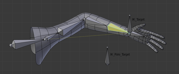
Notez que, si une Pole Target est utilisée, le verrouillage IK ne fonctionnera pas sur le bout racine.