Introduction
Inverse Kinematics (IK) simplifies the animation process, and makes it possible to make more advanced animations with lesser effort.
Inverse Kinematics allow you to position the last bone in a bone chain and the other bones are positioned automatically. This is like how moving someone’s finger would cause their arm to follow it. By normal posing techniques, you would have to start from the root bone, and set bones sequentially until you reach the tip bone: When each parent bone is moved, its child bone would inherit its location and rotation. Thus making tiny precise changes in poses becomes harder farther down the chain, as you may have to adjust all the parent bones first.
This effort is effectively avoided by use of IK.
IK is mostly done with bone constraints although there is also a simple Auto IK feature in Pose Mode. They work by the same method but the constraints offer more options and control. Please refer to the following pages for details about these constraints:
Armature IK Panel
Reference
- Mode:
Pose Mode
- Panel:
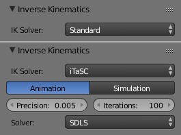
This panel is used to select the IK Solver type for the armature: Standard or iTaSC. Most the time people will use the Standard IK solver.
Standard
Todo
Add this information.
iTaSC
iTaSC stands for instantaneous Task Specification using Constraints.
iTaSC uses a different method to compute the Jacobian, which makes it able to handle other constraints than just end effectors position and orientation: iTaSC is a generic multi-constraint IK solver. However, this capability is not yet fully exploited in the current implementation, only two other types of constraints can be handled: Distance in the Cartesian space, and Joint Rotation in the joint space. The first one allows maintaining an end effector inside, at, or outside a sphere centered on a target position, the second one is the capability to control directly the rotation of a bone relative to its parent. Those interested in the mathematics can find a short description of the method used to build the Jacobian here.
iTaSC accepts a mix of constraints, and multiple constraints per bone: the solver computes the optimal pose according to the respective weights of each constraint. This is a major improvement from the current constraint system where constraints are solved one by one in order of definition so that conflicting constraints overwrite each other.
- Precision
The maximum variation of the end effector between two successive iterations at which a pose is obtained that is stable enough and the solver should stop the iterations. Lower values means higher precision on the end effector position.
- Iterations
The upper bound for the number of iterations.
- Solver
Selects the inverse Jacobian solver that iTaSC will use.
- SDLS
Computes the damping automatically by estimating the level of ‘cancellation’ in the armature kinematics. This method works well with the Copy Pose constraint but has the drawback of damping more than necessary around the singular pose, which means slower movements. Of course, this is only noticeable in Simulation mode.
- DLS
Computes the damping manually which can provide more reactivity and more precision.
- Damping Max
Maximum amount of damping. Smaller values means less damping, hence more velocity and better precision but also more risk of oscillation at singular pose. 0 means no damping at all.
- Damping Epsilon
Range of the damping zone around singular pose. Smaller values means a smaller zone of control and greater risk of passing over the singular pose, which means oscillation.
Note
Damping and Epsilon must be tuned for each armature. You should use the smallest values that preserve stability.
Note
The SDLS solver does not work together with a Distance constraint. You must use the DLS solver if you are going to have a singular pose in your animation with the Distance constraint.
Both solvers perform well if you do not have a singular pose.
Animation
In Animation mode, iTaSC operates like an IK solver: it is stateless and uses the pose from F-Curves interpolation as the start pose before the IK convergence. The target velocity is ignored and the solver converges until the given precision is obtained. Still the new solver is usually faster than the old one and provides features that are inherent to iTaSC: multiple targets per bone and multiple types of constraints.
Simulation
The Simulation mode is the stateful mode of the solver: it estimates the target’s velocity, operates in a ‘true time’ context, ignores rotation from keyframes (except via a joint rotation constraint) and builds up a state cache automatically.
- Reiteration
- Never
The solver starts from the rest pose and does not reiterate (converges) even for the first frame. This means that it will take a few frames to get to the target at the start of the animation.
- Initial
The solver starts from the rest pose and re-iterates until the given precision is achieved, but only on the first frame (i.e. a frame which doesn’t have any previous frame in the cache). This option basically allows you to choose a different start pose than the rest pose and it is the default value. For the subsequent frames, the solver will track the target by integrating the joint velocity computed by the Jacobian solver over the time interval that the frame represents. The precision of the tracking depends on the feedback coefficient, number of substeps and velocity of the target.
- Always
The solver re-iterates on each frame until the given precision is achieved. This option omits most of the iTaSC dynamic behavior: the maximum joint velocity and the continuity between frames is not guaranteed anymore in compensation of better precision on the end effector positions. It is an intermediate mode between Animation and real-time Simulation.
- Auto Step
Use this option if you want to let the solver set how many substeps should be executed for each frame. A substep is a subdivision on the time between two frames for which the solver evaluates the IK equation and updates the joint position. More substeps means more processing but better precision on tracking the targets. The auto step algorithm estimates the optimal number of steps to get the best trade-off between processing and precision. It works by estimation of the nonlinearity of the pose and by limiting the amplitude of joint variation during a substep. It can be configured with next two parameters:
- Min
Proposed minimum substep duration (in second). The auto step algorithm may reduce the substep further based on joint velocity.
- Max
Maximum substep duration (in second). The auto step algorithm will not allow substep longer than this value.
- Steps
If Auto Step is disabled, you can choose a fixed number of substeps with this parameter. Substep should not be longer than 10 ms, which means the number of steps is 4 for a 25 fps animation. If the armature seems unstable (vibrates) between frames, you can improve the stability by increasing the number of steps.
- Feedback
Coefficient on end effector position error to set corrective joint velocity. The time constant of the error correction is the inverse of this value. However, this parameter has little effect on the dynamic of the armature since the algorithm evaluates the target velocity in any case. Setting this parameter to 0 means ‘opening the loop’: the solver tracks the velocity but not the position; the error will accumulate rapidly. Setting this value too high means an excessive amount of correction and risk of instability. The value should be in the range 20-100. Default value is 20, which means that tracking errors are corrected in a typical time of 100-200 ms. The feedback coefficient is the reason why the armature continues to move slightly in Simulation mode even if the target has stopped moving: the residual error is progressively suppressed frame after frame.
- Max Velocity
Indicative maximum joint velocity in radian per second. This parameter has an important effect on the armature dynamic. Smaller value will cause the armature to move slowly and lag behind if the targets are moving rapidly. You can simulate an inertia by setting this parameter to a low value.
Bone IK Panel
Reference
- Mode:
Pose Mode
- Panel:
This panel is used to control how the Pose Bones work in the IK chain.

- IK Stretch
Stretch influence to IK target.
- Lock
Disallow movement around the axis.
- Stiffness
Stiffness around the axis. Influence disabled if using Lock.
- Limit
Limit movement around the axis.
iTaSC Solver
If the iTaSC IK Solver is used, the bone IK panel changes to add these additional parameters.
- Control Rotation
Activates a joint rotation constraint on that bone. The pose rotation computed from Action or UI interaction will be converted into a joint value and passed to the solver as target for the joint. This will give you control over the joint while the solver still tracks the other IK targets. You can use this feature to give a preferred pose for joints (e.g. rest pose) or to animate a joint angle by playing an action on it.
- Weight
The importance of the joint rotation constraint based on the constraints weight in case all constraints cannot be achieved at the same time. For example, if you want to enforce strongly the joint rotation, set a high weight on the joint rotation constraint and a low weight on the IK constraints.
Arm Rig Example
This arm uses two bones to overcome the twist problem for the forearm. IK locking is used to stop the forearm from bending, but the forearm can still be twisted manually by pressing R Y Y in Pose Mode, or by using other constraints.
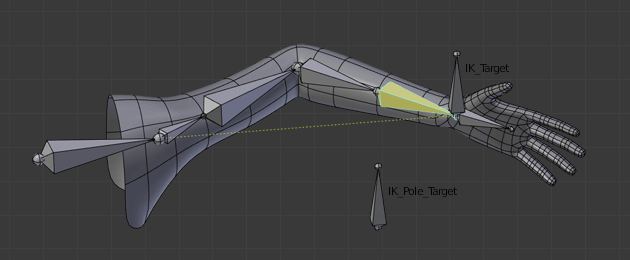
Note that, if a Pole Target is used, IK locking will not work on the root bone.